- Published on
Calculating Measures of Spread Using Python
- Authors
- Name
- Victor Oketch Sabare
- @sabare12


Measures of spread
In this article, I'll talk about a set of summary statistics: measures of spread.
What is spread?
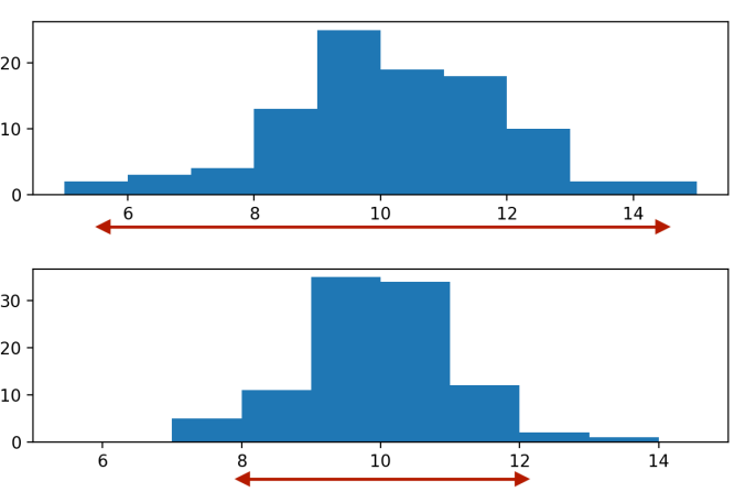
Spread is just what it sounds like - it describes how spread apart or close together the data points are. Just like measures of centre, there are a few different measures of spread.
Variance
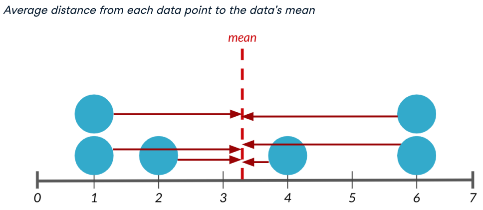
The first measure, variance, measures the average distance from each data point to the data's mean.
Calculating variance
To calculate the variance:
- Subtract the mean from each data point.
dists = msleep['sleep_total'] -
        np.mean(msleep['sleep_total'])
print(dists)
0 1.666265
1 6.566265
2 3.966265
3 4.466265
4 -6.433735
...
So we get one number for every data point.
- Square each distance.
sq_dists = dists ** 2
print(sq_dists)
0   2.776439
1   43.115837
2   15.731259
3  19.947524
4  41.392945
...
- Sum squared distances.
sum_sq_dists = np.sum(sq_dists)
print(sum_sq_dists))
1624.065542
- Divide by the number of data points - 1
variance = sum_sq_dists / (83 - 1)
print(variance)
19.805677
Finally, we divide the sum of squared distances by the number of data points minus 1, giving us the variance. The higher the variance, the more spread out the data is. It's important to note that the units of variance are squared, so in this case, it's 19.8 hours squared. We can calculate the variance in one step using np.var, setting the ddof argument to 1.
np.var(msleep['sleep_total'], ddof=1)
19.805677
If we don't specify ddof equals 1, a slightly different formula is used to calculate variance that should only be used on a full population, not a sample.
np.var(msleep['sleep_total'])
19.567055
Standard deviation
The standard deviation is another measure of spread, calculated by taking the square root of the variance. It can be calculated using np.std, just like np.var, we need to set ddof to 1. The nice thing about standard deviation is that the units are usually easier to understand since they're not squared. It's easier to wrap your head around 4.5 hours than 19.8 hours squared.
np.sqrt(np.var(msleep['sleep_total'], ddof=1))
4.450357
np.std(msleep['sleep_total'], ddof=1)
4.450357
Mean absolute deviation
Mean absolute deviation takes the absolute value of the distances to the mean and then takes the mean of those differences. While this is similar to standard deviation, it's not exactly the same. Standard deviation squares distances, so longer distances are penalized more than shorter ones, while mean absolute deviation penalizes each distance equally. One isn't better than the other, but SD is more common than MAD.
dists = msleep['sleep_total'] - mean(msleep$sleep_total)
np.mean(np.abs(dists))
3.566701
Quantiles
Before we discuss the next measure of spread, let's quickly go through quantiles. Quantiles, also called percentiles, split up the data into some number of equal parts. Here, we call np.quantile, passing in the column of interest, followed by 0.5. This gives us 10.1 hours, so 50% of mammals in the dataset sleep less than 10.1 hours a day, and the other 50% sleep more than 10.1 hours, so this is exactly the same as the median. We can also pass in a list of numbers to get multiple quantiles at once. Here, we split the data into 4 equal parts. These are also called quartiles. This means that 25% of the data is between 1.9 and 7.85, another 25% is between 7.85 and 10.10, and so on.
np.quantile(msleep['sleep_total'], 0.5)
10.1
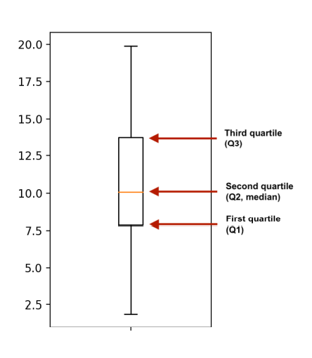
Boxplots use quartiles
The boxes in box plots represent quartiles. The bottom of the box is the first quartile, and the top of the box is the third quartile. The middle line is the second quartile or the median.
import matplotlib.pyplot as plt
plt.boxplot(msleep['sleep_total'])
plt.show()
Quantiles using np.linspace()
Here, we split the data into five equal pieces, but we can also use np.linspace as a shortcut, which takes in the starting number, the stopping number, and the number intervals. We can compute the same quantiles using np.linspace starting at zero, stopping at one, splitting into 5 different intervals.
np.quantile(msleep['sleep_total'], [0, 0.2, 0.4, 0.6, 0.8, 1])
array([ 1.9 , 6.24, 9.48, 11.14, 14.4 , 19.9 ])
np.linspace(start, stop, num)
np.quantile(msleep['sleep_total'], np.linspace(0, 1, 5))
array([ 1.9 , 7.85, 10.1 , 13.75, 19.9 ])
Interquartile range (IQR)
The interquartile range, or IQR, is another measure of spread. It's the distance between the 25th and 75th percentile, which is also the height of the box in a boxplot. We can calculate it using the quantile function, or using the IQR function from scipy.stats to get 5.9 hours.
np.quantile(msleep['sleep_total'], 0.75) - np.quantile(msleep['sleep_total'], 0.25)
5.9
from scipy.stats import iqr
iqr(msleep['sleep_total'])
5.9
Outliers
Outliers are data points that are substantially different from the others. But how do we know what a substantial difference is? A rule that's often used is that any data point less than the first quartile - 1.5 times the IQR is an outlier, as well as any point greater than the third quartile + 1.5 times the IQR.
data < Q1 - 1.5 x IQR or
data > Q3 + 1.5 x IQR
Finding Outliers
To find outliers, we'll start by calculating the IQR of the mammals' body weights. We can then calculate the lower and upper thresholds following the formulas from the previous slide. We can now subset the DataFrame to find mammals whose body weight is below or above the thresholds. There are eleven body weight outliers in this dataset, including the cow and the Asian elephant.
from scipy.stats import iqr
iqr = iqr(msleep['bodywt'])
lower_threshold = np.quantile(msleep['bodywt'], 0.25) - 1.5 * iqr
upper_threshold = np.quantile(msleep['bodywt'], 0.75) + 1.5 * iqr
msleep[(msleep['bodywt'] < lower_threshold) | (msleep['bodywt'] > upper_threshold)]
        name                   vore     sleep_total       bodywt
4      Cow                     herbi         4.0           600.000
20     Asian elephant          herbi         3.9           2547.000
22     Horse                   herbi         2.9           521.00
Using the .describe() method
Many of the summary statistics we've covered so far can all be calculated in just one line of code using the .describe method, so it's convenient to use when you want to get a general sense of your data.
msleep['bodywt'].describe()
count 83.000000
mean 166.136349
std 786.839732
min 0.005000
25% 0.174000
50% 1.670000
75% 41.750000
max 6654.000000
Name: bodywt, dtype: float64